Interactive Topic Modeling with BERTopic
Every day, businesses deal with large volumes of unstructured text. From customer interactions in emails to online feedback and reviews. To deal with this large amount of text, we look towards topic modeling. A technique to automatically extract meaning from documents by identifying recurrent topics.
A few months ago, I wrote an article on leveraging BERT for topic modeling. It blew up unexpectedly and I was surprised by the positive feedback I had gotten!
I decided to focus on further developing the topic modeling technique the article was based on, namely BERTopic.
BERTopic is a topic modeling technique that leverages BERT embeddings and a class-based TF-IDF to create dense clusters allowing for easily interpretable topics whilst keeping important words in the topic descriptions.
I am now at a point where BERTopic has gotten enough traction and development that I feel confident it can replace or complement other topic modeling techniques, such as LDA.
The main purpose of this article is to give you an in-depth overview of BERTopic’s features and tutorials on how to best apply this for your own projects.
1. Installation
As always, we start by installing the package via pypi:
pip install bertopic
To use the visualization options, install BERTopic as follows:
pip install bertopic[visualization]
2. Basic Usage
Using BERTopic out-of-the-box is quite straightforward. You load in your documents as a list of strings and simply pass it to the fit_transform method.
To give you an example, below we will be using the 20 newsgroups dataset:
from bertopic import BERTopic
from sklearn.datasets import fetch_20newsgroups

docs = fetch_20newsgroups(subset='all',  remove=('headers', 'footers', 'quotes'))['data']

model = BERTopic()
topics, probabilities = model.fit_transform(docs)
There are two outputs generated, topics and probabilities. A value in topics simply represents the topic it is assigned to. Probabilities on the other hand demonstrate the likelihood of a document falling into any of the possible topics.
Next, we can access the topics that were generated by their relative frequency:
>>>> model.get_topic_freq().head()
Topic   Count
-1      7288
49      3992
30      701
27      684
11      568
In the output above, it seems that Topic -1 is the largest. -1 refers to all outliers which do not have a topic assigned. Forcing documents in a topic could lead to poor performance. Thus, we ignore Topic -1.
Instead, let us take a look at the second most frequent topic that was generated, namely Topic 49:
>>>> model.get_topic(49)
[('windows', 0.006152228076250982),
 ('drive', 0.004982897610645755),
 ('dos', 0.004845038866360651),
 ('file', 0.004140142872194834),
 ('disk', 0.004131678774810884),
 ('mac', 0.003624848635985097),
 ('memory', 0.0034840976976789903),
 ('software', 0.0034415334250699077),
 ('email', 0.0034239554442333257),
 ('pc', 0.003047105930670237)]
Since I created this model, I am obviously biased, but to me, this does seem like a coherent and easily interpretable topic!
Languages
Under the hood, BERTopic is using sentence-transformers to create embeddings for the documents you pass it. As a default, BERTopic is set to using an English model but is supports any language for which an embedding model exists.
You can choose the language by simply setting the language parameter in BERTopic:
from bertopic import BERTopic
model = BERTopic(language="Dutch")
When you select a language, the corresponding sentence-transformers model will be loaded. This is typically a multilingual model that supports many languages.
Having said that, if you have a mixture of language in your documents you can use BERTopic(language="multilingual") to select a model that supports over 50 languages!
Embedding model
To chose a different pre-trained embedding model, we simply pass it through BERTopic by pointing the variable embedding_model towards the corresponding sentence-transformers model:
from bertopic import BERTopic
model = BERTopic(embedding_model="xlm-r-bert-base-nli-stsb-mean-tokens")
Click here for a list of supported sentence transformers models.
Save/Load BERTopic model
We can easily save a trained BERTopic model by calling save:
from bertopic import BERTopic
model = BERTopic()
model.save("my_model")
Then, we can load the model in one line:
loaded_model = BERTopic.load("my_model")
3. Visualization
Now that we have covered the basics and generated our topics, we visualize them! Having an overall picture of the topics allows us to generate an internal perception of the topic model’s quality.
Visualize Topics
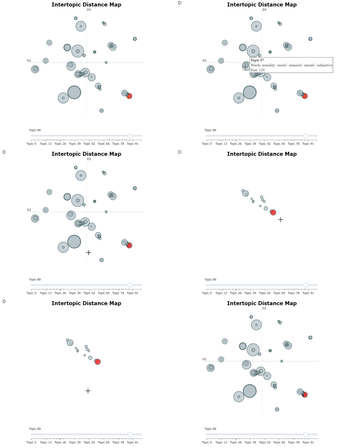
To visualize our topics I took inspiration from LDAvis which is a framework for visualizing LDA topic models. It allows you to interactively explore topics and the words that describe them.
To achieve a similar effect in BERTopic, I embedded our class-based TF-IDF representation of the topics in 2D using Umap. Then, it was a simple matter of visualizing the dimensions using Plotly to create an interactive view.
To do this, simply call model.visualize_topics() in order to visualize our topics:

An interactive Plotly figure will be generated which can be used as indicated in the animation above. Each circle indicates a topic and its size is the frequency of the topic across all documents.
To try it out yourself, take a look at the documentation here where you can find an interactive version!
Visualize Probabilities
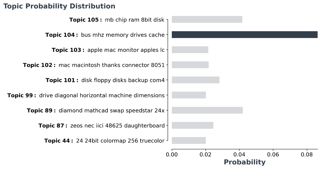
For each document, we can also visualize the probability of that document belong to each possible topic. To do so, we use the variable probabilities after running BERTopic to understand how confident the model is for that instance.
Since there are too many topics to visualize, we visualize the probability distribution of the most probable topics:
model.visualize_distribution(probabilities[0])

It seems that for this document, the model had some more difficulty choosing the correct topic as they were multiple topics very similar to each other.
4. Topic Reduction
As we have seen before, hundreds of topics could be generated. At times, this might simply be too much for you to explore or a too fine-grained solution.
Fortunately, we can reduce the number of topics by merging pairs of topics that are most similar to each other, as indicated by the cosine similarity between c-TF-IDF vectors.
Below, I will go into three methods for reducing the number of topics that result from BERTopic.
Manual Topic Reduction
When initiating your BERTopic model, you might already have a feeling of the number of topics that could reside in your documents.
By setting the nr_topics variable, BERTopic will find the most similar pairs of topics and merge them, starting from the least frequent topic, until we reach the value of nr_topics:
from bertopic import BERTopic
model = BERTopic(nr_topics=20)
It is advised, however, to keep a decently high value, such as 50 to prevent topics from being merged that should not.
Automatic Topic Reduction
As indicated above, if you merge topics to a low nr_topics topics will be forced to merge even though they might not actually be that similar to each other.
Instead, we can reduce the number of topics iteratively as long as a pair of topics is found that exceeds a minimum similarity of 0.9.
To use this option, we simply set nr_topics to "auto" before training our model:
from bertopic import BERTopic
model = BERTopic(nr_topics="auto")
Topic Reduction after Training
What if you are left with too many topics after training which took many hours? It would be a shame to have to re-train your model just to experiment with the number of topics.
Fortunately, we can reduce the number of topics after having trained a BERTopic model. Another advantage of doing so is that you can decide the number of topics after knowing how many are actually created:
from bertopic import BERTopic

model = BERTopic()
topics, probs = model.fit_transform(docs)

# Further reduce topics
new_topics, new_probs = model.reduce_topics(docs, topics, probs, nr_topics=30)
Using the code above, we reduce the number of topics to 30 after having trained the model. This allows you to play around with the number of topics that suit your use-case!
5. Topic Representation
Topics are typically represented by a set of words. In BERTopic, these words are extracted from the documents using a class-based TF-IDF.
At times, you might not be happy with the representation of the topics that were created. This is possible when you selected to have only 1-gram words as representation. Perhaps you want to try out a different n-gram range or you have a custom vectorizer that you want to use.
To update the topic representation after training, we can use the function update_topics to update the topic representation with new parameters for c-TF-IDF:
# Update topic representation by increasing n-gram range and removing english stopwords
model.update_topics(docs, topics, n_gram_range=(1, 3), stop_words="english")
We can also use a custom CountVectorizer instead:
from sklearn.feature_extraction.text import CountVectorizer

cv = CountVectorizer(ngram_range=(1, 3), stop_words="english")
model.update_topics(docs, topics, vectorizer=vectorizer)
6. Custom Embeddings
Why limit ourselves to publicly available pre-trained embeddings? You might have very specific data for which you have created an embedding model that you could not have found pre-trained available.
Transformer Models
To use any embedding model that you trained yourself, you will only have to embed your documents with that model. You can then pass in the embeddings and BERTopic will do the rest:
from bertopic import BERTopic
from sentence_transformers import SentenceTransformer

# Prepare embeddings
sentence_model = SentenceTransformer("distilbert-base-nli-mean-tokens")
embeddings = sentence_model.encode(docs, show_progress_bar=False)

# Create topic model
model = BERTopic()
topics, probabilities = model.fit_transform(docs, embeddings)
As you can see above, we used a SentenceTransformer model to create the embedding. You could also have used 🤗 transformers, Doc2Vec, or any other embedding method.
TF-IDF
While we are at it, why limit ourselves to transformer models? There is a reason why statistical models, such as TF-IDF, are still around. They work great out-of-the-box without much tuning!
As you might have guessed, it is also possible to use TF-IDF on the documents and use them as input for BERTopic. We simply create a TF-IDF matrix and pass it through fit_transform:
from bertopic import BERTopic
from sklearn.feature_extraction.text import TfidfVectorizer

# Create TF-IDF sparse matrix
vectorizer = TfidfVectorizer(min_df=5)
embeddings = vectorizer.fit_transform(docs)

# Model
model = BERTopic(stop_words="english")
topics, probabilities = model.fit_transform(docs, embeddings)
Here, you will probably notice that creating the embeddings is quite fast whereas fit_transform is quite slow. This is to be expected as reducing the dimensionality of a large sparse matrix takes some time. The inverse of using transformer embeddings is true: creating the embeddings is slow whereas fit_transform is quite fast.